estimate

Signature/Parameters

class estimate
def __init__(self, G, formula = None, data = None, model = 'auto', family = 'auto', se_cluster = None, se = None, model_kws = {}, weights = 1, *args, **kws)

Structural Equation Model (SCM) estimation of Graphical Causal Models (GCM).

Parameters:

Name	Type	Description	Default
G	DAG	Causal graph describing relationships among observed and latent variables created by causalinf.gcm.DAG.	required
model		Models for the functions of the structural causal model. “auto” : use LSEM (default) “LSEM”: Estimate (parametric) generalized linear structural equation models. “NPSEM-IE-BART: Estimate nonparametric structural equation models with independent errors using BART. “NPSEM-IE-GAM: Estimate nonparametric structural equation models with independent errors using GAM.	'auto'
formula	str or None	Formula for the functional form of the SCM. The formula depends on the model used and defined by the argument model. If None it creates a formula automatically based on the model used. Auto-generated formulas do not include interactions between variables in the DAG. If model='auto', the formula generated includes definitions for direct, indirect, and total effect parameters whenever exposure/outcome roles are defined in the DAG object provided to the G argument. To provide custom formulas: If model='LSEM' or model='auto': Use the formula format as used for the sem() function of R’s lavaan. For additional model-specific documentation, see causalinf.models.lsem. If model='NPSEM-IE-BART': TBD For additional model-specific documentation, see causalinf.models.bart. If model='NPSEM-IE-GAM': TBD For additional model-specific documentation, see causalinf.models.gam.	None
data	DataFrame - like	Observational dataset containing all variables referenced by the DAG or formula.	None
family	str	Outcome distribution family. Defaults to 'auto', in which case the family is infered from the type of outcome in the data.	'auto'
se_cluster	str	Name of the variable to cluster the std. errors.	None
se	str or None	Options available depend on the model used. See comments in formula to find model-specific documentation and model-specific options for se. See also Notes below.	None
model_kws	dict	Additional keyword arguments for the model defined in model. The accepted arguments for each respective model are those accepted by the function described in formula. See also Notes below.	{}
weights	str or array - like	Observation weights passed through to the estimator. Defaults to 1 (equal weights).	1
*args		Additional positional arguments forwarded to the underlying estimator.	()
**kws		Additional keyword arguments forwarded to the underlying estimator.	{}

Notes

For documentation of model-specific arguments, see:

• LSEM: ‘causalinf.models.lsem‘
• NPSEM-IE-BART: ‘causalinf.models.bart‘
• NPSEM-IE-GAM: ‘causalinf.models.gam‘

Attributes:

Name	Type	Description
G	DAG	Original DAG used in the estimation.
formula	str	SEM specification employed during fitting.
fit	object	Raw estimator output (e.g., lavaan fit object) when available.
est	dict	Summary bundle returned by the selected estimator, including parameter tables, fit statistics, and option metadata.

Examples:

>>> dag = gcm.DAG("X -> Y")
>>> data = tp.tibble({'X': [0, 1, 0], 'Y': [1.0, 2.5, 1.2]})
>>> est = estimate(G=dag, data=data, silent=True)
>>> est.est['fit']['N_obs']
3

Source code in causalinf/scm.py

class estimate:
    """
    Structural Equation Model (SCM) estimation of Graphical Causal Models (GCM).

    Parameters
    ----------
    G : gcm.DAG
        Causal graph describing relationships among observed and latent
        variables created by ``causalinf.gcm.DAG``.

    model: str
        Models for the functions of the structural causal model.

        * "auto" : use LSEM (default)
        * "LSEM": Estimate (parametric) generalized linear structural equation models. 
        * "NPSEM-IE-BART: Estimate nonparametric structural equation
                    models with independent errors using BART. 
        * "NPSEM-IE-GAM: Estimate nonparametric structural equation
                    models with independent errors using GAM. 

    formula : str or None, optional
        Formula for the functional form of the SCM. The formula depends on the
        model used and defined by the argument ``model``.
        If ``None`` it creates a formula automatically based on the
        ``model`` used. Auto-generated formulas do not include interactions
        between variables in the DAG. 
        If ``model='auto'``, 
        the formula generated includes definitions for direct, indirect,
        and total effect parameters whenever exposure/outcome roles are defined
        in the DAG object provided to the ``G`` argument. To provide custom formulas:

        * If ``model='LSEM'`` or ``model='auto'``: Use the formula format as used for the ``sem()`` function of R's lavaan.
          For additional model-specific documentation, see ``causalinf.models.lsem``.
        * If ``model='NPSEM-IE-BART'``:  TBD
          For additional model-specific documentation, see ``causalinf.models.bart``.
        * If ``model='NPSEM-IE-GAM'``:  TBD
          For additional model-specific documentation, see ``causalinf.models.gam``.

    data : DataFrame-like
        Observational dataset containing all variables referenced by the DAG or
        formula. 

    family : str, optional
        Outcome distribution family. Defaults to ``'auto'``, in which
        case the family is infered from the type of outcome in the data.
    se_cluster : str
        Name of the variable to cluster the std. errors. 
    se : str or None
        Options available depend on the ``model`` used. See comments in
        ``formula`` to find model-specific documentation and model-specific
        options for ``se``. See also ``Notes`` below.
    model_kws : dict, optional
        Additional keyword arguments for the model defined in ``model``.
        The accepted arguments for each respective ``model`` are those accepted
        by the function described in ``formula``. See also ``Notes`` below.
    weights : str or array-like, optional
        Observation weights passed through to the estimator. Defaults to
        ``1`` (equal weights).
    *args :
        Additional positional arguments forwarded to the underlying estimator.
    **kws :
        Additional keyword arguments forwarded to the underlying estimator.


    Notes
    -----
    For documentation of model-specific arguments, see:

    * LSEM: '``causalinf.models.lsem``'
    * NPSEM-IE-BART: '``causalinf.models.bart``'
    * NPSEM-IE-GAM: '``causalinf.models.gam``'

    Attributes
    ----------
    G : gcm.DAG
        Original DAG used in the estimation.
    formula : str
        SEM specification employed during fitting.
    fit : object
        Raw estimator output (e.g., lavaan fit object) when available.
    est : dict
        Summary bundle returned by the selected estimator, including parameter
        tables, fit statistics, and option metadata.

    Examples
    --------
    >>> dag = gcm.DAG("X -> Y")
    >>> data = tp.tibble({'X': [0, 1, 0], 'Y': [1.0, 2.5, 1.2]})
    >>> est = estimate(G=dag, data=data, silent=True)
    >>> est.est['fit']['N_obs']
    3
    """
    def __init__(self,
                 G,
                 formula=None,
                 data=None,
                 model='auto',
                 family = 'auto',
                 se_cluster=None,
                 se=None,
                 # 
                 model_kws={},
                 # 
                 weights=1,
                 *args,
                 **kws
                 ):
        assert data is not None, 'Data must be provided.'
        data = ut.data2tibble(data)
        self.model = "LSEM" if model=='auto' else model
        self.formula = formula or self._graph2sem(G)
        self.family = family
        # 
        self.G = G
        self.outcome = G.outcome[0]
        self.exposure =G.exposure
        #
        self.se_cluster = se_cluster
        self.se = se

        if self.model in 'LSEM':
            self._lsem(G, data=data, weights=weights, *args, **kws)

    @ut.copy_docstring(lsem)
    def _lsem(self, G, data, weights, *args, **kws):
        est =  lsem(formula=self.formula,
                    data=data,
                    weights=weights,
                    se=self.se,
                    se_cluster=self.se_cluster,
                    *args, **kws)
        self.fit = est.fit
        self.est = est.est

    @property
    def causalinf(self):
        print(self)

    @ut.copy_docstring(ut.summary)
    def summary(self, *args, **kws):
        formula = ("\n" + self.formula).replace('\n', '\n        ')
        kws |= {'formula': kws.get("formula", formula)}

        latex_replace = {"~~": "\\\\leftrightarrow ", "~" : "\\\\leftarrow "}
        kws |= {'latex_replace': kws.get("latex_replace", latex_replace)}

        res = ut.summary(
            model = self,
            id_strategy='SCM',
            *args, **kws
        )
        return res.res

    def get_fit_statsitics(self, stats):
        res = self.est['fit_stats'].get(stats, None)
        if res is None:
            print(f'Statistics {stats} not available.')
        return res

    @ut.copy_docstring(gcm.DAG.plot)
    def plot(self, *args, **kws):
        self.G.plot(estimates=self, *args, **kws)

    def _graph2sem(self, G, parameter_fmt="(beta_{cause}.{effect})"):
        # regression lines
        reg = ''
        for y, pa_y in G.nodes_parents.items():
            pa_y = " + ".join([f"(beta_{v}.{y})*{v}" for v in pa_y])
            reg += f"{y} ~ (beta_0{y})*1 + {pa_y}\n"
        reg = f"# LSEM:\n{reg}"

        # correlations
        corr = "\n".join([f"{n1[0]} ~~ {n2[0]}" for n1, n2 in G.bidirected])
        corr += "\n".join([f"{n1} ~~ {n2}" for n1, n2 in G.undirected])
        if corr:
            corr = f"# Correlations:\n{corr}"

        # indirect effects
        if G.exposure and G.outcome:
            ind = self._graph2sem_indirect_and_total_effects(G, parameter_fmt)
        else:
            ind = ''

        sem = f"{reg}{corr}{ind}"
        return sem

    def _graph2sem_indirect_and_total_effects(self, G, parameter_fmt):
        # """
        # edges    : list of (u, v) directed edges
        # exposure, outcome : compute indirect paths from exposure to outcome
        # parameter_fmt: how to name each coefficient (e.g., 'beta_{u}.{v}' or '(beta_{u}.{v})')
        # returns  : list of (path_nodes, effect_str)
        # """
        # build adjacency
        edges = G.directed
        exposure = G.exposure[0]
        outcome = G.outcome[0]

        adj = defaultdict(list)
        for u, v in edges:
            adj[u].append(v)

        dir_effect = []
        tot_effect = []
        ind_effects = []

        # direct effect
        if outcome in adj[exposure]:
            dir_effect = parameter_fmt.format(cause=exposure, effect=outcome)

        # enumerate simple paths (DFS) recursive function
        def dfs(node, visited, path):
            if node == outcome and len(path) >= 3:  # indirect: at least 2 edges
                # build product beta terms for edges along the path
                terms = [parameter_fmt.format(cause=path[i], effect=path[i+1]) for i in range(len(path)-1)]
                ind_effects.append( (path[:], " * ".join(terms)) )
                return
            for nxt in adj[node]:
                if nxt in visited:       # avoid cycles
                    continue
                visited.add(nxt)
                path.append(nxt)
                dfs(nxt, visited, path)
                path.pop()
                visited.remove(nxt)
        # this wil fill in the info and save it in the variable ind_effects
        dfs(exposure, {exposure}, [exposure])

        res = ''
        ind_effect_str = ''
        if ind_effects:
            for i, ind in enumerate(ind_effects):
                parameter = f"Indirect_effect_{i+1}" # f"beta_{'.'.join(ind[0])}"
                ind_effect_str += f"{parameter} := {ind[1]}\n"
                tot_effect += [parameter]
            res += f"# Indirect effects:\n{ind_effect_str}"
        if dir_effect:
            parameter = "Direct_effect"
            res += f"# Direct effect:\n{parameter} := {dir_effect}"
            tot_effect += [parameter]
        if tot_effect:
            res += f"\n# Total effect:\nTotal_effect := {' + '.join(tot_effect)}"

        return res

    def __repr__(self):
        self.summary(style="full")
        return ''

Examples

Estimate LSEM

Take this GCM example:

from causalinf import gcm
from causalinf import scm
from causalinf import simulate

G = gcm.examples('Two confounders')
G.plot()

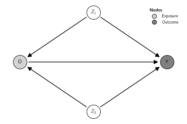
Simulate a data from a LSEM based on that DAG:

sim = simulate.lsem(G, seed=10)
df = sim.data
df.head().print()

shape: (5, 4)
┌───────────────────────────────┐
│    Z1      Z2       D       Y │
│   f64     f64     f64     f64 │
╞═══════════════════════════════╡
│  1.33    1.51   -2.58    0.50 │
│  0.72   -0.14   -0.42   -1.39 │
│ -1.55   -0.14    1.08   -0.59 │
│ -0.01    1.18   -0.90   -0.47 │
│  0.62    1.18    0.22    0.07 │
└───────────────────────────────┘

Estimat the model:

res = scm.estimate(G, data=df)
print(res)

Estimating LSEM...done!

================================================================================
Model: Model 1
Identification: SCM
Outcome: Y
Exposure: D
Formula: 
# LSEM:
D ~ (beta_0D)*1 + (beta_Z1.D)*Z1 + (beta_Z2.D)*Z2
Y ~ (beta_0Y)*1 + (beta_D.Y)*D + (beta_Z1.Y)*Z1 + (beta_Z2.Y)*Z2
# Direct effect:
Direct_effect := (beta_D.Y)
# Total effect:
Total_effect := Direct_effect
Summary:
--------        
 term                  label          estimate    sig  se      lo       hi       statistic  pvalue 
 D ~ 1                 beta_0D        0.3129      ***  0.0312  0.2518   0.374    10.0358    0.0    
 D ~ Z1                beta_Z1.D      -0.8867     ***  0.0333  -0.952   -0.8214  -26.6224   0.0    
 D ~ Z2                beta_Z2.D      -0.9231     ***  0.0314  -0.9847  -0.8616  -29.3942   0.0    
 Y ~ 1                 beta_0Y        -0.2967     ***  0.0333  -0.3619  -0.2315  -8.9172    0.0    
 Y ~ D                 beta_D.Y       0.0179           0.0322  -0.0451  0.081    0.5571     0.5775 
 Y ~ Z1                beta_Z1.Y      -0.0581          0.0443  -0.1449  0.0287   -1.312     0.1895 
 Y ~ Z2                beta_Z2.Y      0.1846      ***  0.0436  0.0991   0.2701   4.2314     0.0    
 D ~~ D                               0.9715      ***  0.0434  0.8863   1.0566   22.3607    0.0    
 Y ~~ Y                               1.0054      ***  0.045   0.9173   1.0935   22.3607    0.0    
 Z1 ~~ Z1                             0.8798           0.0     0.8798   0.8798   --         --     
 Z1 ~~ Z2                             0.0632           0.0     0.0632   0.0632   --         --     
 Z2 ~~ Z2                             0.9896           0.0     0.9896   0.9896   --         --     
 Z1 ~ 1                               -0.0146          0.0     -0.0146  -0.0146  --         --     
 Z2 ~ 1                               -0.0111          0.0     -0.0111  -0.0111  --         --     
 Direct_effect := (be  Direct_effect  0.0179           0.0322  -0.0451  0.081    0.5571     0.5775 
 Total_effect := Dire  Total_effect   0.0179           0.0322  -0.0451  0.081    0.5571     0.5775 
 Model                 --             (footnote)  --   --      --       --       --         --     
 Outcome type          --             (footnote)  --   --      --       --       --         --     
 Estimator             --             ML          --   --      --       --       --         --     
 Std.Error             --             classic     --   --      --       --       --         --     
 N.obs                 --             1000        --   --      --       --       --         --     
 RMSE                  --             0.0         --   --      --       --       --         --     
 AIC                   --             5670.18     --   --      --       --       --         --     
 BIC                   --             5714.35     --   --      --       --       --         --     
 DF (model)            --             0           --   --      --       --       --         --     
================================================================================
*** p<0.001; ** p<0.01; * p<0.05; + p<0.1
Model 1: Endogenous variable types: Continuous (D, Y); Models: Linear (D, Y)